The Ultimate Guide: Streamlining Complex QGIS Topographical Data Exports for Industrial SCADA Mapping in Water Infrastructure
Master the integration of QGIS topographical data into industrial SCADA systems with this comprehensive step-by-step guide for water infrastructure managers. Learn how to streamline complex shapefile conversions, optimize coordinate reference systems, and automate geospatial exports for high-performance mapping.
- The Challenge of GIS-to-SCADA Integration in water Infrastructure
- Step-by-Step Troubleshooting and Optimization Guide
- Step 1: Resolving Coordinate Reference System (CRS) Conflicts
- Step 2: Geometry Simplification to Prevent HMI Freezes
- Step 3: Automating the Export Process via PyQGIS
- Step 4: SCADA Ingestion and Custom Parsing
- Step 5: Telemetry Overlay and Validation
- Export Format Comparison for SCADA Integration
- Conclusion
The Challenge of GIS-to-SCADA Integration in water Infrastructure
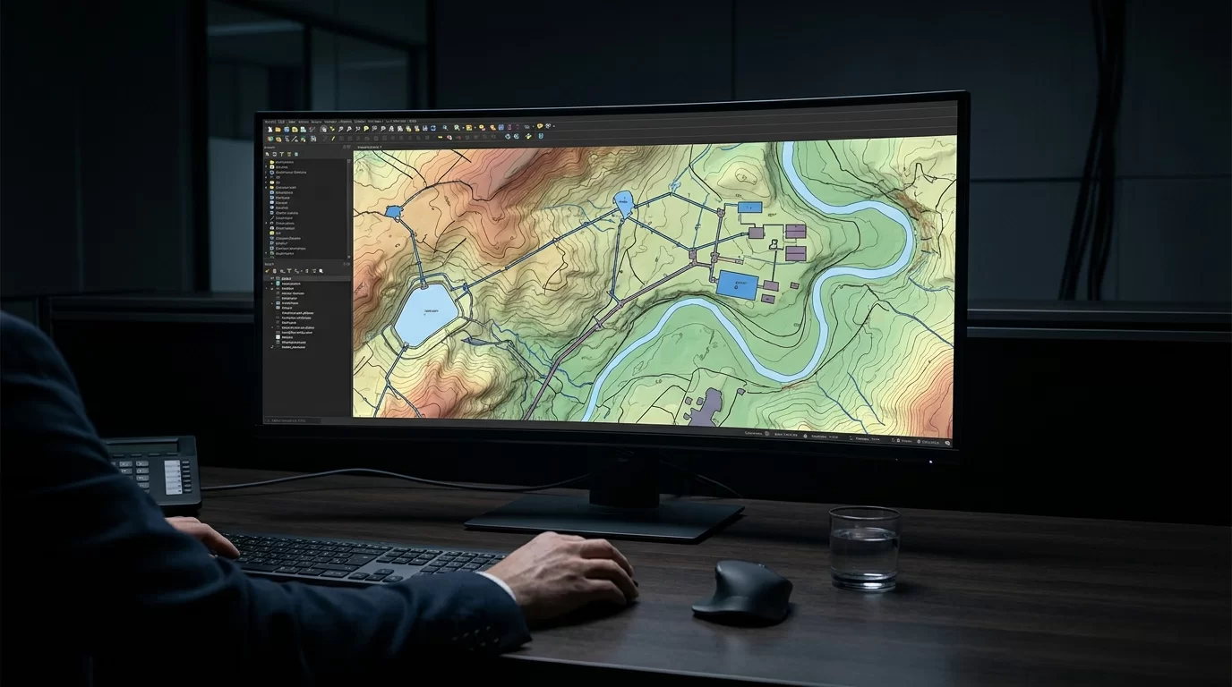
For water Infrastructure Managers, bridging the gap between high-fidelity Geographic Information Systems (GIS) and real-time Supervisory Control and Data Acquisition (SCADA) platforms is a notorious operational hurdle. QGIS is the industry standard for managing complex topographical data—such as elevation contours, pipeline networks, and reservoir boundaries. However, SCADA Human-Machine Interfaces (HMIs) are optimized for real-time telemetry, not for rendering millions of geospatial vertices. When raw QGIS shapefiles are dumped directly into SCADA mapping components, the result is often severe HMI latency, memory crashes, and sluggish operator response times.
As a Field Automation Engineer, I frequently encounter SCADA systems crippled by unoptimized GIS data. This guide provides a step-by-step technical troubleshooting workflow to streamline complex QGIS exports, ensuring your SCADA mapping remains highly responsive while providing operators with critical topographical context.
Step-by-Step Troubleshooting and Optimization Guide
Step 1: Resolving Coordinate Reference System (CRS) Conflicts
The Problem: SCADA mapping engines (like those in Ignition, GeoSCADA, or Reliance) typically expect data in WGS 84 (EPSG:4326) or Web Mercator (EPSG:3857). water utilities often maintain QGIS data in localized projected coordinate systems (e.g., State Plane or UTM) for precise physical measurements. Exporting without CRS transformation causes SCADA assets to appear in the ocean or fail to render entirely.
The Fix: Before exporting, you must standardize the CRS.
- Open your QGIS project and right-click the target layer (e.g., ‘Main_Distribution_Pipes’).
- Navigate to Export > Save Features As…
- In the CRS dropdown, explicitly select EPSG:4326 – WGS 84. Do not rely on the default project CRS.
- If your SCADA system utilizes tile servers (like OpenStreetMap), verify if EPSG:3857 is preferred to prevent micro-misalignments between your vector lines and the base map.
Step 2: Geometry Simplification to Prevent HMI Freezes
The Problem: A 50-mile pipeline shapefile might contain 500,000 vertices. SCADA clients will attempt to render every single node, consuming massive amounts of RAM and CPU, leading to frozen screens during pan/zoom operations.
The Fix: Implement geometry thinning using the Douglas-Peucker algorithm.
- In QGIS, open the Processing Toolbox (Ctrl+Alt+T).
- Search for and open the Simplify tool.
- Select your pipeline or contour layer.
- Set the tolerance. For pipeline overviews in SCADA, a tolerance of 1 to 5 meters is usually sufficient and can reduce vertex count by up to 90% without compromising visual accuracy on an HMI screen.
- Save the output as a new temporary layer for the final export.
Step 3: Automating the Export Process via PyQGIS
Manual exports are prone to human error and are unsustainable for dynamic water networks where infrastructure is continuously updated. To ensure your SCADA system always has the latest topographical data, you should automate the filtering, CRS transformation, and export process using a Python (PyQGIS) script. This script grabs the active layer, simplifies it, reprojects it, and outputs a lightweight GeoJSON file perfectly formatted for SCADA ingestion.
import os
from qgis.core import (
    QgsProject,
    QgsVectorFileWriter,
    QgsCoordinateReferenceSystem,
    QgsCoordinateTransformContext,
    QgsGeometry
)

# Configuration
LAYER_NAME = 'Water_Mains_Raw'
OUTPUT_PATH = 'C:/SCADA_Exports/Water_Mains_Optimized.geojson'
TARGET_CRS = QgsCoordinateReferenceSystem('EPSG:4326')
SIMPLIFY_TOLERANCE = 2.5 # Meters (assuming source CRS is metric)

def export_for_scada():
    # 1. Fetch the layer
    layer = QgsProject.instance().mapLayersByName(LAYER_NAME)
    if not layer:
        print(f"Error: Layer {LAYER_NAME} not found.")
        return
    layer = layer[0]

    # 2. Setup export options for GeoJSON
    options = QgsVectorFileWriter.SaveVectorOptions()
    options.driverName = "GeoJSON"
    options.fileEncoding = "utf-8"
    options.ct = QgsCoordinateTransformContext()
    options.destCRS = TARGET_CRS

    # 3. Filter out unnecessary attributes to reduce file size
    # Only keep 'Pipe_ID' and 'Diameter'
    fields = layer.fields()
    keep_indices = [fields.indexOf('Pipe_ID'), fields.indexOf('Diameter')]
    options.attributes = [idx for idx in keep_indices if idx != -1]

    # 4. Execute Export
    error, msg = QgsVectorFileWriter.writeAsVectorFormatV3(
        layer,
        OUTPUT_PATH,
        QgsProject.instance().transformContext(),
        options
    )

    if error == QgsVectorFileWriter.NoError:
        print(f"Success! Optimized SCADA mapping data saved to {OUTPUT_PATH}")
    else:
        print(f"Export failed: {msg}")

export_for_scada()
Step 4: SCADA Ingestion and Custom Parsing
Once you have your optimized GeoJSON or CSV file, the SCADA system needs to parse and render it. While modern platforms have native map components, legacy or highly customized environments might require custom backend scripts to translate this spatial data into internal SCADA tags or database tables. If you are dealing with complex data ingestion from remote sites, you might find it beneficial to read our guide on developing high-performance C# data parsers for non-standard IoT sensors, as the principles of parsing complex JSON payloads apply directly to handling geospatial data streams.
Step 5: Telemetry Overlay and Validation
The final step is binding live telemetry to your newly imported GIS data. A map of pipelines is useless without live pressure and flow data. Overlay your SCADA tags onto the GIS coordinates. If you are using this spatial data to feed advanced simulation engines, ensure your geospatial nodes match your telemetry nodes. For a deeper dive into this synchronization, check out our tutorial on calibrating real-time hydraulic models using live Reliance SCADA telemetry.
Export Format Comparison for SCADA Integration
Choosing the right export format from QGIS is critical for SCADA performance. Below is a technical comparison of standard formats used in water infrastructure mapping.
| Export Format | SCADA Compatibility | File Size / Overhead | Best Use Case in water Infrastructure |
|---|---|---|---|
| GeoJSON | Excellent (Modern web-based HMIs like Ignition Perspective) | Medium (Text-based, easily compressed) | Dynamic pipeline rendering and real-time asset tracking. |
| Shapefile (SHP) | Moderate (Requires specific legacy GIS modules) | High (Multiple files, binary overhead) | Static, offline mapping where the SCADA system has a dedicated GIS server. |
| Well-Known Text (WKT) | High (Easily stored in standard SQL databases) | Low (Highly efficient string representation) | Storing individual pump station or valve coordinates in a SCADA SQL backend. |
| KML | Low to Moderate (Often requires conversion) | High (XML bloat) | Quickly sharing topographical overlays with field technicians using Google Earth. |
Conclusion
Integrating QGIS topographical data into your industrial SCADA system does not have to result in sluggish HMIs and frustrated operators. By strictly standardizing your Coordinate Reference Systems, aggressively simplifying geometries, automating exports via PyQGIS, and selecting the optimal file format, water Infrastructure Managers can achieve high-fidelity, zero-latency situational awareness. Implement these steps to ensure your control room has the exact geospatial context needed to manage critical water distribution networks efficiently.